OutlierDetection.rst

Outlier Detection and Flagging

The tutorial aims to introduce the usage of saqc methods in order to detect outliers in an uni-variate set up. The tutorial guides through the following steps:

1. We checkout and load the example data set. Subsequently, we initialise an :py:class:`SaQC <saqc.core.core.SaQC>` object.
   • :ref:`Preparation <cookbooks/OutlierDetection:Preparation>`
     • :ref:`Data <cookbooks/OutlierDetection:Data>`
     • :ref:`Initialisation <cookbooks/OutlierDetection:Initialisation>`
2. We will see how to apply different smoothing methods and models to the data in order to obtain usefull residual variables.
   • :ref:`Modelling <cookbooks/OutlierDetection:Modelling>`
     • :ref:`Rolling Mean <cookbooks/OutlierDetection:Rolling Mean>`
     • :ref:`Rolling Median <cookbooks/OutlierDetection:Rolling Median>`
     • :ref:`Polynomial Fit <cookbooks/OutlierDetection:Polynomial Fit>`
     • :ref:`Custom Models <cookbooks/OutlierDetection:Custom Models>`
   • :ref:`Evaluation and Visualisation <cookbooks/OutlierDetection:Visualisation>`
3. We will see how we can obtain residuals and scores from the calculated model curves.
   • :ref:`Residuals and Scores <cookbooks/OutlierDetection:Residuals and Scores>`
     • :ref:`Residuals <cookbooks/OutlierDetection:Residuals>`
     • :ref:`Scores <cookbooks/OutlierDetection:Scores>`
     • :ref:`Optimization by Decomposition <cookbooks/OutlierDetection:Optimization by Decomposition>`
4. Finally, we will see how to derive flags from the scores itself and impose additional conditions, functioning as correctives.
   • :ref:`Setting and Correcting Flags <cookbooks/OutlierDetection:Setting and Correcting Flags>`
     • :ref:`Flagging the Scores <cookbooks/OutlierDetection:Flagging the Scores>`
     • Additional Conditions ("unflagging")
     • :ref:`Including Multiple Conditions <cookbooks/OutlierDetection:Including Multiple Conditions>`

Preparation

Data

The example data set is selected to be small, comprehendable and its single anomalous outlier can be identified easily visually:

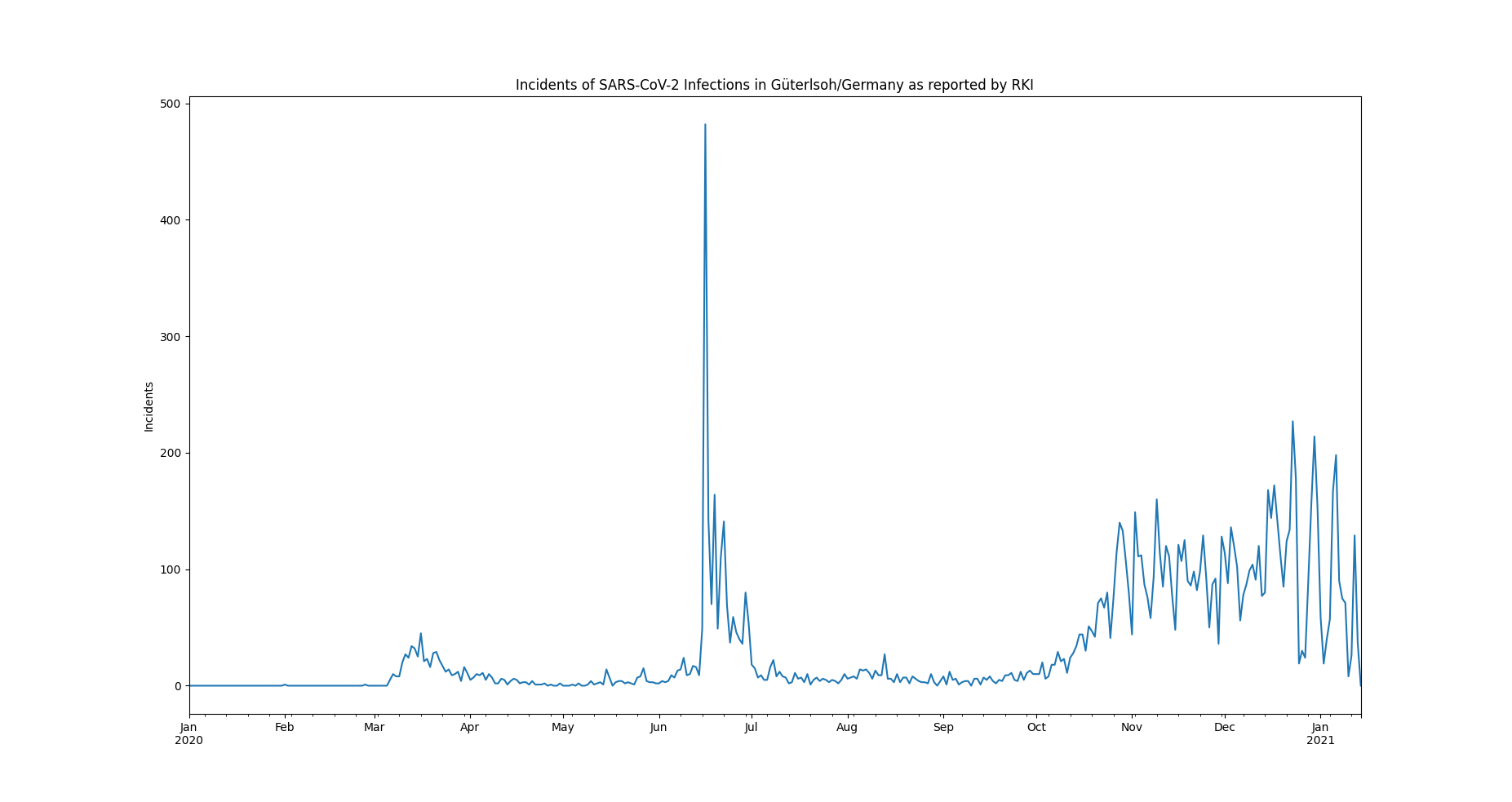
It can be downloaded from the saqc git repository.

The data represents incidents of SARS-CoV-2 infections, on a daily basis, as reported by the RKI in 2020.

In June, an extreme spike can be observed. This spike relates to an incidence of so called "superspreading" in a local meat factory.

For the sake of modelling the spread of Covid, it can be of advantage, to filter the data for such extreme events, since they may not be consistent with underlying distributional assumptions and thus interfere with the parameter learning process of the modelling. Also it can help to learn about the conditions severely facilitating infection rates.

To introduce into some basic saqc workflows, we will concentrate on classic variance based outlier detection approaches.

Initialisation

We initially want to import the data into our workspace. Therefore we import the pandas library and use its csv file parser pd.read_csv.

>>> data_path = './resources/data/incidentsLKG.csv'
>>> import pandas as pd
>>> data = pd.read_csv(data_path, index_col=0)

The resulting data variable is a pandas data frame object. We can generate an :py:class:`SaQC <saqc.core.core.SaQC>` object directly from that. Beforehand we have to make sure, the index of data is of the right type.

>>> data.index = pd.DatetimeIndex(data.index)

Now we do load the saqc package into the workspace and generate an instance of :py:class:`SaQC <saqc.core.core.SaQC>` object, that refers to the loaded data.

>>> import saqc
>>> qc = saqc.SaQC(data)

The only timeseries have here, is the incidents dataset. We can have a look at the data and obtain the above plot through the method :py:meth:`~saqc.SaQC.plot`:

>>> qc.plot('incidents') # doctest: +SKIP

Modelling

First, we want to model our data in order to obtain a stationary, residuish variable with zero mean.

Rolling Mean

Easiest thing to do, would be, to apply some rolling mean model via the method :py:meth:`saqc.SaQC.roll`.

>>> import numpy as np
>>> qc = qc.roll(field='incidents', target='incidents_mean', func=np.mean, window='13D')

The field parameter is passed the variable name, we want to calculate the rolling mean of. The target parameter holds the name, we want to store the results of the calculation to. The window parameter controlls the size of the rolling window. It can be fed any so called date alias string. We chose the rolling window to have a 13 days span.

Rolling Median

You can pass arbitrary function objects to the func parameter, to be applied to calculate every single windows "score". For example, you could go for the median instead of the mean. The numpy library provides a median function under the name np.median. We just calculate another model curve for the "incidents" data with the np.median function from the numpy library.

>>> qc = qc.roll(field='incidents', target='incidents_median', func=np.median, window='13D')

We chose another :py:attr:`target` value for the rolling median calculation, in order to not override our results from the previous rolling mean calculation. The :py:attr:`target` parameter can be passed to any call of a function from the saqc functions pool and will determine the result of the function to be written to the data, under the fieldname specified by it. If there already exists a field with the name passed to target, the data stored to this field will be overridden.

We will evaluate and visualize the different model curves :ref:`later <cookbooks/OutlierDetection:Visualisation>`. Beforehand, we will generate some more model data.

Polynomial Fit

Another common approach, is, to fit polynomials of certain degrees to the data. :py:class:`SaQC <Core.Core.SaQC>` provides the polynomial fit function :py:meth:`~saqc.SaQC.fitPolynomial`:

>>> qc = qc.fitPolynomial(field='incidents', target='incidents_polynomial', order=2, window='13D')

It also takes a :py:attr:`window` parameter, determining the size of the fitting window. The parameter, :py:attr:`order` refers to the size of the rolling window, the polynomials get fitted to.

Custom Models

If you want to apply a completely arbitrary function to your data, without pre-chunking it by a rolling window, you can make use of the more general :py:meth:`~saqc.SaQC.process` function.

Lets apply a smoothing filter from the scipy.signal module. We wrap the filter generator up into a function first:

This function object, we can pass on to the :py:meth:`~saqc.SaQC.processGeneric` methods func argument.

>>> qc = qc.processGeneric(field='incidents', target='incidents_lowPass', func=lambda x: butterFilter(x, cutoff=0.1, nyq=0.5, filter_order=2))